A list of projects that I have completed throughout my classes.
Neuropsychiatric Symptoms in Late Onset Alzheimer’s Disease & Down Syndrome Alzheimer’s Disease
Currently ongoing.
Weather Data Candle Plot
This was my final project in my INFO 474 course Interactive Information Visualization. The goal of the project was to use weather data and create a completely different plot that answered a specific user question.
The user question that my candle plot answered was related to a weather forecaster attempting to ascertain the maximum, minimum, and average temperatures for a modifiable date range.
The visualization is coded in HTML, CSS, and Javascript. A viewer can click and drag on the plot area to zoom in to a certain date range, and can double click anywhere to zoom back out. The drop down menu can be used to switch between different cities’ weather data. Finally, the top of the candle is the maximum temperature for that day, the bottom of the candle is the minimum temperature for that day, and the black line is the average temperature for that day. The candle is red if the maximum temperature is greater than the minimum temperature, and blue for the opposite.
This was my final group project in my STAT 342 course Introduction to Probability and Mathematical Statistics III. The goal of the project was to create and use Method of Moments (MOM) and Maximum Likelihood Estimators (MLE) to find out the efficacy of the BNT162b2 COVID-19 vaccine.
The was my final group project in my INFO 330 course Client-Side Web Development. The purpose of the project was to create an interactive web application, for which my group and I created a fitness and workout app that allows for users to log in and record both their food intake and workouts.
This web application was coded in HTML, CSS, and Javascript, and was then hosted on Firebase. The link to this app is here: Health & Fitness Tracker.
LGBTQIA+ Cartoon Analysis
This was my final group project in my INFO 201 course Foundational Skills for Data Science. The aim of the project was to analyze the presence of LGBTQIA+ characters in children’s cartoons.
This analysis contains three interactive visualizations, which are coded in R as a Shiny app. The link to the Shiny app is: LGBTQIA+ Cartoon Analysis Shiny App.
Fish Population Analysis
This was my final group project in my AMATH 383 course Introduction to Continuous Mathematical Modeling. The goal of this project was to measure the accuracy of the base logistical model against actual fish populations over time.
This was my final project in my INFO 330 course Data and Data Modeling. The goal of this project was to create a complicated database and then answer user queries for said database. This database of Nintendo video games and game bundles as well as the resulting user queries are coded in SQL.
The proposal document for the project, which outlines the information needs for the database as well as the main entities, is linked here: Nintendo SQL Database Proposal Document.
The Excel database that I manually created to represent the various Nintendo games is linked here: Nintendo SQL Excel Database.
The Phase 1 Entity-Relationship Diagram (ERD), along with the Phase 2 Relational Schema for the database are additionally linked below:
The final project file that includes a summary of the database as well as all of the user queries and their respective results is linked here: Nintendo SQL Database Final Project Summary.
Statistics Directed Reading Program 2023
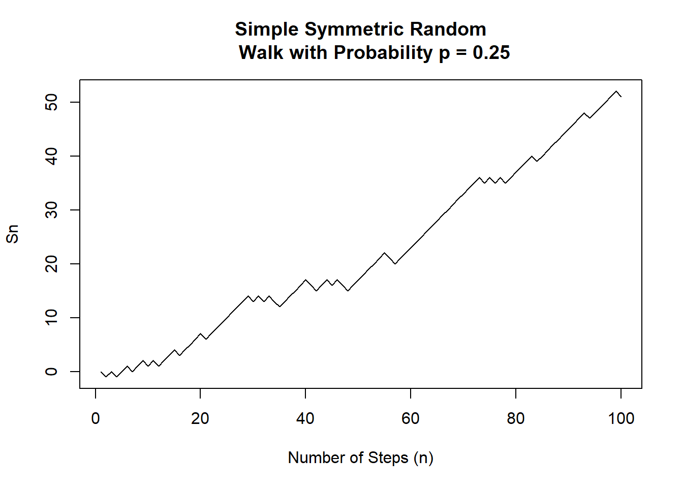
This was the project that I completed during the Statistics Directed Reading Program in my 2023 spring quarter at the University of Washington. I was taught about the topic of random walks from a graduate student and then presented what I learned to a group of fellow students from the directed reading program as well as statistics professors.
Below is my summary document of what I understood as well as the presentation that I presented to my fellow students and the statistics professors:
Additionally, below is my R code for graphically demonstrating random walks as well as calculating their convergence:
#install.packages("igraph")#install.packages("expm")library(expm)library(igraph)# First set up a symmetric random walksym_walk <-function(x0, n){ values <-c(0) current <- x0while (length(values) < n) { change =0if (runif(1) >0.5) { change =1 }else { change =-1 } current <- current + change values <-c(values, current) } values}plot(sym_walk(0, 100), xlab ="Number of Steps (n)",ylab ="Sn", main ="Simple Symmetric Random Walk with Probability p = 0.5", type ="l")
# Second set up a random walk without symmetryprob_walk <-function(x0, p, n){ values <-c(0) current <- x0while (length(values) < n) { change =0if (runif(1) > p) { change =1 }else { change =-1 } current <- current + change values <-c(values, current) } values}plot(prob_walk(0, 0.25, 100), xlab ="Number of Steps (n)", ylab ="Sn", main ="Simple Symmetric Random Walk with Probability p = 0.25", type ="l")
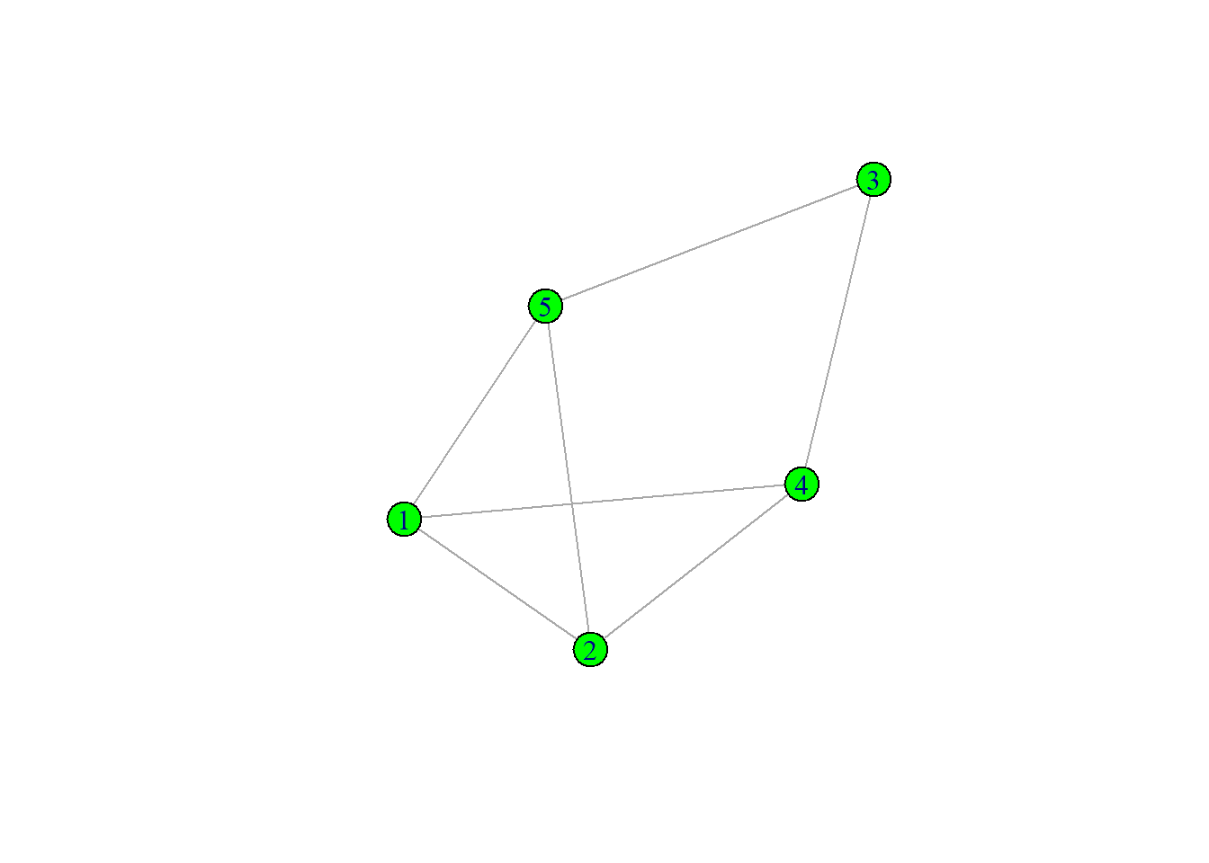
# Third graph random walk on graph w/ equal probG <-make_graph(~1-2, 3-4, 4-1:2, 5-1:2:3)plot(G, vertex.color ="green")
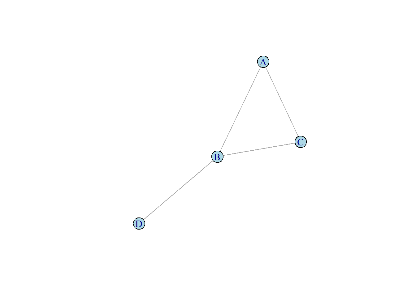
# Degree Matrix of Graph Gdeg <-degree(G)G_deg <-diag(deg, 5, 5)# Adjacency Matrix of Graph GG_adj <-matrix(as_adj(G), byrow =FALSE, nrow =5)# Manually Computed LaplacianG_man_lap <- G_deg - G_adj# Computer Computed LaplacianG_com_lap <-matrix(laplacian_matrix(G), byrow =FALSE, nrow =5)# Manually Computed Normalized Laplaciandeg_neg_half <-degree(G)^(-0.5)G_deg_neg_half <-diag(deg_neg_half, 5, 5)G_man_norm_lap <- G_deg_neg_half %*% G_man_lap %*% G_deg_neg_half# Computer Computer Normalized LaplacianG_com_norm_lap <-matrix(laplacian_matrix(G, normalized =TRUE), byrow =FALSE, nrow =5)# That proves the Laplacian matrix as well as our# equation to normalize it.# Now to do some stuff with the original M matrixH <-make_graph(~ A - B:C, B - C:D)plot(H, vertex.color ="light blue")
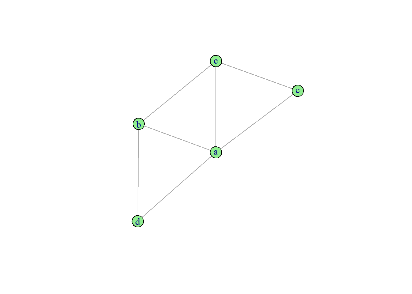
trans_prob_step <-function(graph, t){ nodes =vcount(graph) d <-degree(graph) M <-matrix(0, nodes, nodes)for (i in1:nodes) {for (j in1:nodes) {if (are_adjacent(graph, i, j) ==TRUE) { M[i, j] =1/d[i] }else { M[i, j] =0 } } }if (t ==0) {print("Invalid Operation.") }elseif (t ==1) { M <- M }else {for (k in1:(t-1)) { M <- M %*% M } } N <- M}N <-trans_prob_step(H, 2)prob_cloud <-function(graph, t, i){ A <-trans_prob_step(graph, t) v <- A[i,] v}row <-prob_cloud(H, 2, 1)lazy_matrix_step <-function(graph, t){ nodes =vcount(graph) d <-degree(graph) M <-matrix(0, nodes, nodes)if (runif(1) >0.5) {for (i in1:nodes) {for (j in1:nodes) {if (are_adjacent(graph, i, j) ==TRUE) { M[i, j] =1/d[i] }else { M[i, j] =0 } } } }else { M <-diag(nodes) }if (t >=2) { k =1while (k < t) { S <-matrix(0, nodes, nodes)if (runif(1) >0.5) {for (i in1:nodes) {for (j in1:nodes) {if (are_adjacent(graph, i, j) ==TRUE) { S[i, j] =1/d[i] }else { S[i, j] =0 } } } }else { S <-diag(nodes) } M = M %*% S k = k +1 } } A <- M}L <-lazy_matrix_step(H, 2)I <-make_graph(~ a - b, c - a:b, d - a:b, e - a:c)plot(I, vertex.color ="light green")
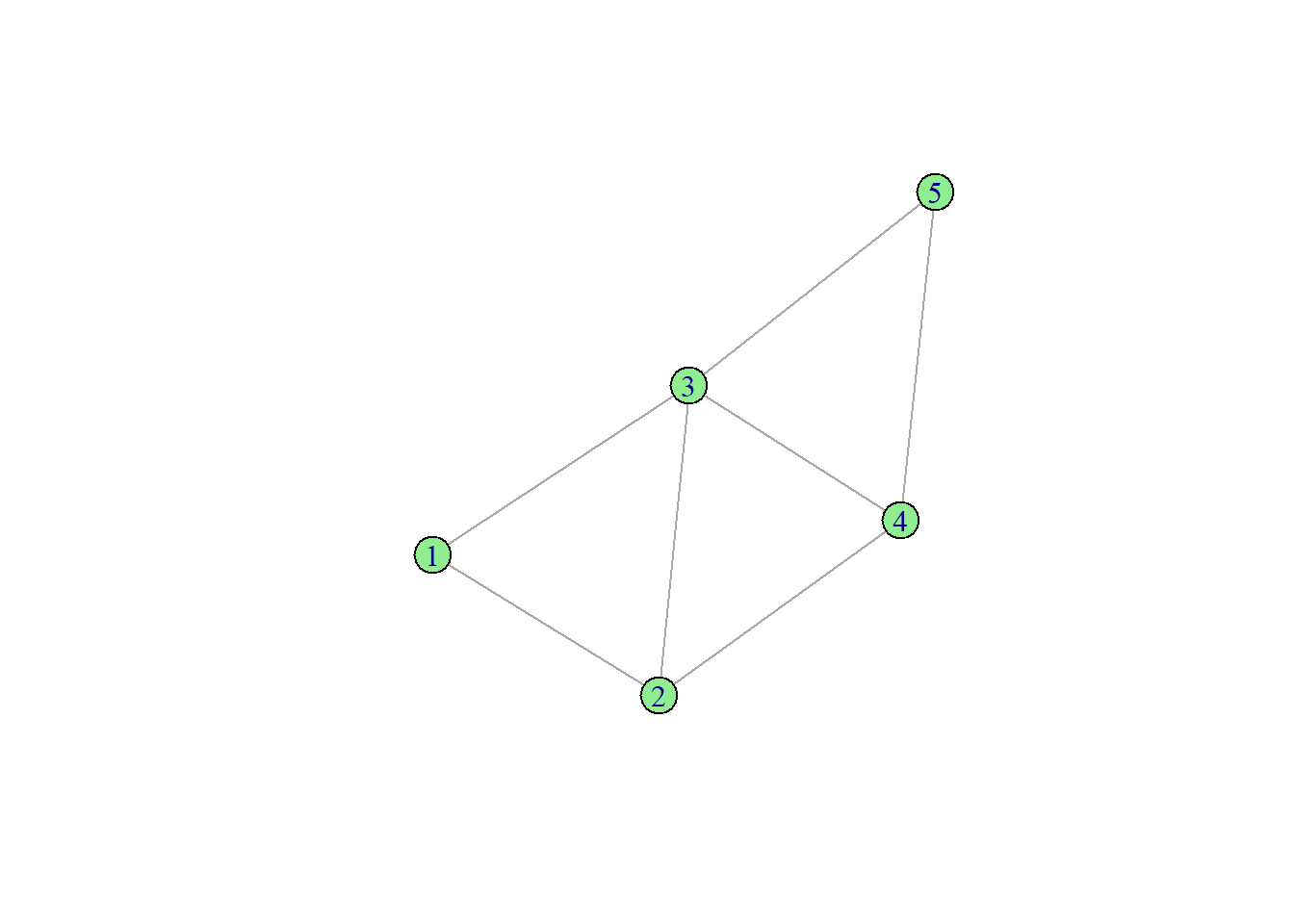
convergence <-function(graph){ nodes =vcount(graph) val =1 R <-trans_prob_step(graph, val)while ((R[1, 1] + R[2, 1]) != (2* R[1, 1])) { val = val +1 R <-trans_prob_step(graph, val) } val}num <-convergence(I)converg_matrix <-function(graph){ t <-convergence(graph) R <-trans_prob_step(graph, t) R}decomp_trans_prob <-function(graph, p){ M <-trans_prob_step(graph, 1) nodes =vcount(graph) deg <-degree(graph) D <-diag(deg, nodes, nodes) half_D <-diag(degree(graph)^(0.5), nodes, nodes) neg_half_D <-diag(degree(graph)^(-0.5), nodes, nodes) S <- half_D %*% M %*% neg_half_D evs <-eigen(S) evals <- evs$values evects <- evs$vectors lambda <-diag(evals, nodes, nodes) phi <- neg_half_D %*% evects psi <- half_D %*% evects E <-matrix(0, nodes, nodes)for (a in1:nodes) { r <-t(t(phi[,a])) y <-t(psi[,a]) E <- E + ((evals[a]^p) * r %*% y) } E <-round(E, digits =7)}E <-decomp_trans_prob(H, 2)M <-trans_prob_step(H, 2)J <-make_graph(~1-2:3, 2-3:4, 3-4:5, 4-5)plot(J, vertex.color ="light green")
F <-converg_matrix(J)power <-convergence(J)P <-trans_prob_step(J, 9)